8 Time-Saving Microsoft Excel Formulas for Efficiency

Microsoft Excel, used the right way, is an exceptional tool for analyzing and manipulating data. Knowing the right Microsoft Excel formulas that can help you will really speed up your time also boost your career prospects in various fields, including marketing, finance, and project management. Strong Excel skills can be particularly valuable for creating compelling LinkedIn portfolios. In this post, we will consider the 8 essential Microsoft Excel formulas that will increase your efficiency with explanations and visual examples so that it can be understood better.

1. SUMIF: Quickly Calculate Totals Based on Criteria

The SUMIF Microsoft Excel formula is useful in computing the summation of values, depending on a particular criterion. This function is quite versatile because it allows one to get the sum of values given certain predefined factors. Be it by product, region, or date, the SUMIF will help in fast aggregation of information of interest. It’s a must-have for anyone working with numerical data in Excel. It takes three arguments:

SUMIF Formula:

=SUMIF(range, criteria, [sum_range])

• Range: The range of cells to be evaluated.
• Criteria: The condition to be met.
• Sum_range: The range of cells to be summed.

Key points:

• Calculates the sum of values based on a specific criterion.
• Takes three arguments: range, criteria, and sum_range.
• Can use text, numbers, or logical expressions for criteria.
• Supports wildcards (* and ?) for more flexible matching.

For Example, to sum only sales figures from “Region A,” you would use:

=SUMIF(B2:B10, “north”, C2:C10)

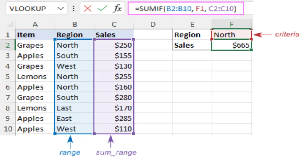
This formula is used to get a total sales of North region.

2. COUNTIF: Count Cells Meeting a Specific Condition

The COUNTIF function counts cells of a certain range based on some given criterion. Another important function in data analysis is the COUNTIF function. It counts the number of cells in a range that satisfy some condition. This can be very useful to know the frequency of different occurrences or outliers in your data. It takes two arguments:

COUNTIF Formula:

=COUNTIF(range, criteria)

• Range: The range of cells to be evaluated.
• Criteria: The condition to be met.

Key points:

• Counts the number of cells within a range that meet a specific criterion.
• Takes two arguments: range and criteria.
• Can use text, numbers, or logical expressions for criteria.
• Supports wildcards for more flexible matching.

For instance, to count the number of orders placed after a specific date:

=COUNTIF(D5:D16,”>100″)

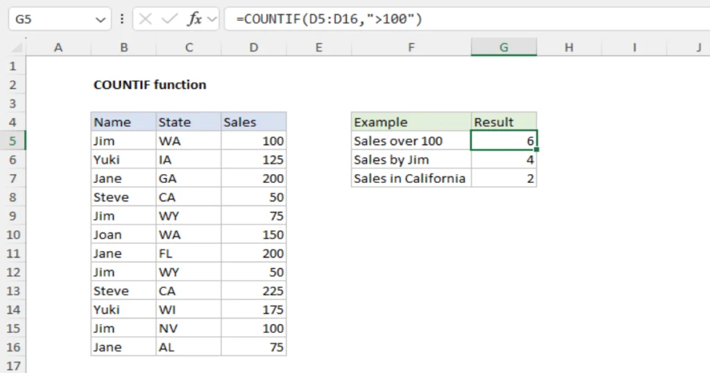
This formula counts numbers greater than 100 in the range D5:D16.

3. VLOOKUP: Look Up Values in a Table

The VLOOKUP Microsoft Excel formula allows for finding a value within a table and returning the value corresponding to that searched in another column. Using the VLOOKUP function, one is able to look up information on the basis of a value within a table. It is mainly applied in matching data with a unique identifier. You can use it to find the price of the product you want by using a product code. It takes four arguments:

VLOOKUP Formula:

=VLOOKUP(lookup_value, table_array, col_index_num, [range_lookup])

• Lookup_value: The value to search for.
• Table_array: The range of cells containing the table.
• Col_index_num: The column number from which to return the value.
• Range_lookup: Specifies whether to find an exact match (FALSE) or an approximate match (TRUE).

Key points:

• Looks up a value in a table and returns a corresponding value from a different column.
• Takes four arguments: lookup_value, table_array, col_index_num, and range_lookup.
• range_lookup can be TRUE for approximate match or FALSE for exact match.
• Useful for data retrieval and analysis.

For example, we want to know Sandra Kwon’s employee ID based on her last name:

=VLOOKUP(B6,B2:D10,3,FALSE)

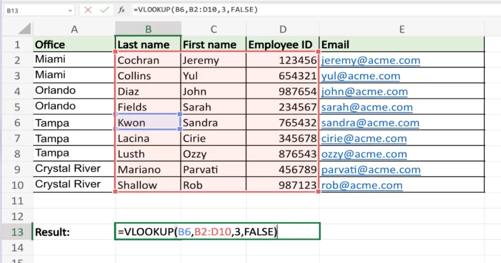
This formula looks up to know Sandra Kwon’s employee ID based on her last name. 

4. CONCATENATE: Combine Text Strings

Use CONCATENATE to join multiple text strings into a single cell. It takes multiple arguments, each representing a text string to be combined. The CONCATENATE function works well with the concatenation of string text. Among other common uses are in cases when one needs to create custom labels or bring data together from several columns. For instance, use CONCATENATE to glue first and last names into a full name.

CONCATENATE Formula:

=CONCATENATE(text1, text2, ...)

Key points:

• Joins multiple text strings into a single string.
• Takes multiple arguments, each representing a text string to be combined.
• Can be used to create custom labels or combine data from different columns.

For instance, to combine a first name and last name:

=CONCATENATE(A2,B2)

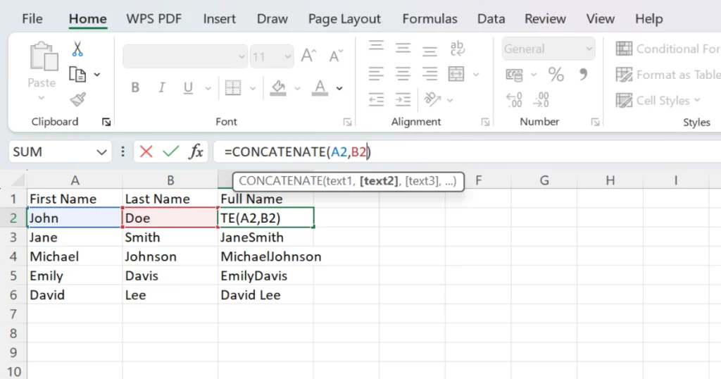
This formula joins the values in cells A2 and B2.

5. IF: Perform Logical Tests

IF is the very basic Excel function applied for running a conditional statement. It does different things depending on whether certain conditions are true or false. This can help in making a dynamic, interactive spreadsheet. It takes three arguments:

IF Formula:

=IF(test, value_if_true, value_if_false)

• Test: The logical expression to be evaluated.
• Value_if_true: The value to return if the test is true.
• Value_if_false: The value to return if the test is false.

Key points:

• The function conducts a logical test and returns one of the values depending on the test result.
• It takes three arguments: test, value_if_true and value_if_false.
• It can be used in generating conditional statements and decision-making logic.

For Example, let’s write a very simple IF formula that checks a value in cell A2 and returns “Good” if the value is greater than 80, “Bad” otherwise:

=IF(B2>80, “Good”, “Bad”)

This formula returns “Good” if the value in cell B2 is greater than 80, otherwise it returns “Bad.”

6. AVERAGEIF: Calculate Averages Based on Criteria

Use the AVERAGEIF function when you need to determine an average of numbers that satisfies a certain condition. The AVERAGEIF function does all that the function SUMIF does, but instead, it gets the average. This would be applicable if one were to find out the average of the value from a set of data satisfying a condition. It takes three arguments:

AVERAGEIF Formula:

=AVERAGEIF(range, criteria, [average_range])

• Range: The range of cells to be evaluated.
• Criteria: The condition to be met.
• Average_range: The range of cells to be averaged.

Key points:

• Calculates the average of values based on a specific criterion.
• Takes three arguments: range, criteria, and average_range.
• Similar to SUMIF, but calculates the average instead of the sum.

For example, to average the numbers in column B if column A contains “Apple”, the formula is:

=AVERAGEIF(A3:A15, F3, B3:B15)

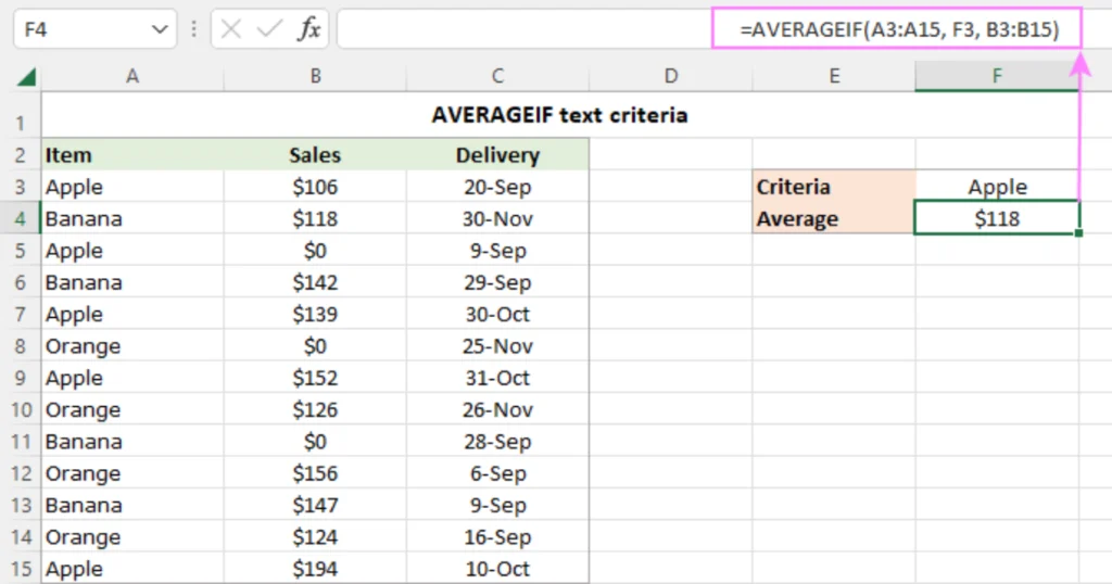
This formula calculates the average numbers in column B if column A contains “Apple”.

7. INDEX-MATCH: Flexible Lookups

The combination of INDEX and MATCH is much more flexible than VLOOKUP. You can not only look up values by row criteria but also by column criteria. This combination of the INDEX and MATCH functions presents a very powerful alternative to using VLOOKUP. It is capable of doing a lot more and handling many scenarios that would otherwise be too complex for VLOOKUP; chief among these are non-sequential criteria.

INDEX-MATCH Formula:

=INDEX(array, row_num, [column_num]) and =MATCH(lookup_value, lookup_array, [match_type])

• INDEX returns a value from a range based on row and column numbers.
• MATCH finds the position of a value within a range.

Key points:

• A powerful combination for flexible lookups.
• INDEX returns a value from a range based on row and column numbers.
• MATCH finds the position of a value within a range.
• Offers more flexibility than VLOOKUP for complex lookup scenarios.

For example, to find the sales for a specific Seller and month:

=VLOOKUP(H4,B5:E16,MATCH(H5,B4:E4,0),0)

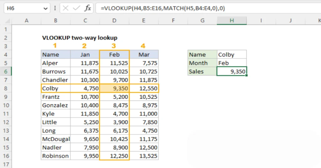
Cell H4 provides the lookup value for the row “Colby”, and cell H5 supplies the lookup value for the column “Feb”. The result is 9,350, the value for Colby in February.

8. Pivot Tables: Summarize and Analyze Data

Pivot tables are extremely useful for summarizing and analyzing large data sets. They enable a user to form, quickly, cross-tabulations and compute several metrics. Pivot tables help in quickly summarizing and analyzing large data volumes. They enable the user to form, in a quick way, cross-tabulations, calculate several metrics, and look at the data from many different angles. In other words, pivot tables are core to data exploration and reporting.

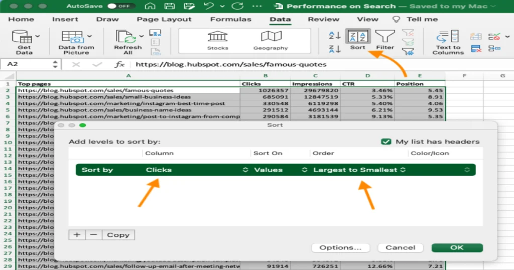
First, select the data you want to turn into a pivot table. Then go to the Data tab and click Sort. You are asked to select a location for the PivotTable. Drag and drop fields onto areas below: in the Field List pane, in the areas of Row Labels, Column Labels, and Values.

Key points:

• A tool for summarizing and analyzing large datasets.
• Allows you to create cross-tabulations and calculate various metrics.
• Drag and drop fields to create different views of your data.
• Useful for data exploration and reporting.

Conclusion

Master these 8 key Microsoft Excel formulas, and you will be improving your overall productivity and efficiency. The excel formulas will range in function from simple calculations to advanced data analysis. Experiment with how they can help smooth out workflows and save a great deal of time.

Practice is key to mastering these formulas. Experiment with different datasets and scenarios to solidify your understanding. With consistent practice, you’ll be able to confidently apply these formulas to your own projects and unlock the full potential of Excel.

Frequently Asked Questions: